This page is part of a larger series on Path Planning, where the corresponding github repository can be found here. This project specifically demonstrates using Rapidly Exploring Random Trees in a small example, implemented in MATLAB. The corresponding sub-repository can be found here.
Table Of Contents
Motion Planning for robotics consists of moving a robot from a start state to a goal state while avoiding obstacles as well as obeying constraints such as joint and torque limits.

Path Planning is a subset of the larger field of Motion Planning. Path planning consists of finding the geometric path that connects a start state to a goal state, while avoiding obstacles. In path planning, however, we ignore robot dynamics and additional environmental and motion constraints.
In this project, we will be exploring Rapidly Exploring Random Trees for path planning. If you're interested in other projects in this Path Planning series, check out my page on A* Search Algorithm.
Much like in the A* Search Algorithm, we begin by creating an environment with a START node, a GOAL node, as well as OBSTACLES.
Here is what our example environment will look like:
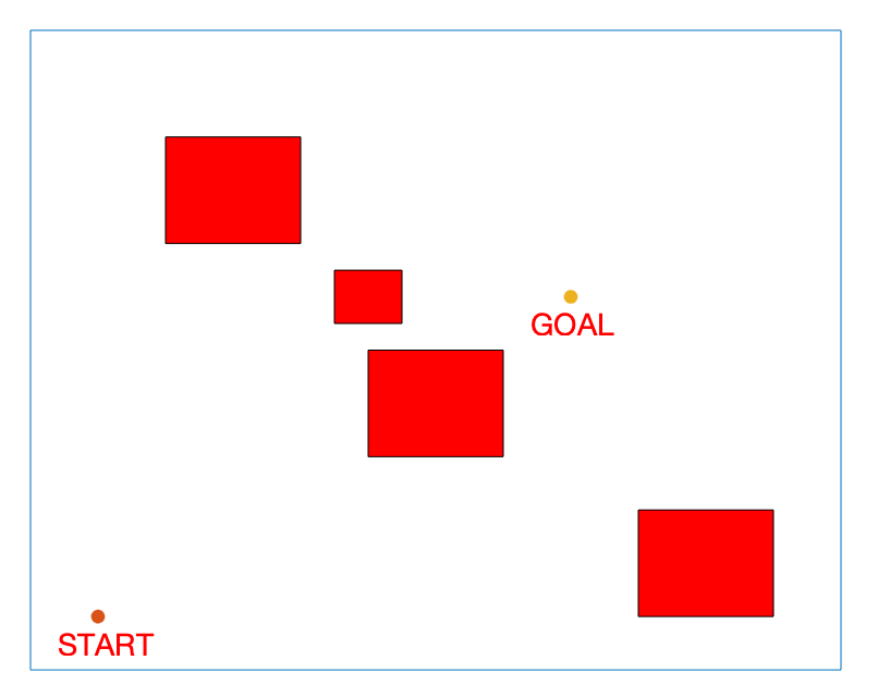
And here is the section of the code that creates and plots this environment:
OB = [0 0; 12 0; 12 12; 0 12; 0 0];
qs = [1 1];
qg = [8 7];

figure
plot(OB(:,1),OB(:,2))
hold on
plot(qs(1), qs(2), '.', 'MarkerSize', 20)
text(qs(1)-0.6,qs(2)-0.5,'START','Color','red','FontSize',14)
plot(qg(1), qg(2), '.', 'MarkerSize', 20)
text(qg(1)-0.6,qg(2)-0.5,'GOAL','Color','red','FontSize',14)
axis([-1 13 -1 13])

obstacle = [5 4; 7 4; 7 6; 5 6; 5 4];
obstacle2 = [4.5 6.5; 5.5 6.5; 5.5 7.5; 4.5 7.5; 4.5 6.5];
obstacle3 = [2 8; 4 8; 4 10; 2 10; 2 8];
obstacle4 = [9 1; 11 1; 11 3; 9 3; 9 1];
obstacle5 = [7 2; 8 2; 8 3; 7 3; 7 2];

fill(obstacle(:,1), obstacle(:,2),'r')
fill(obstacle2(:,1), obstacle2(:,2),'r')
fill(obstacle3(:,1), obstacle3(:,2),'r')
fill(obstacle4(:,1), obstacle4(:,2),'r')
fill(obstacle5(:,1), obstacle5(:,2),'r')
You can easily change the positions of the START and GOAL nodes as well as the number and positions of the OBSTACLES here.
In general, the RRT algorithm has two goals:
- Find a path from the
STARTnode to theENDnode - Explore the space
Unlike the A* algorithm, the RRT does not guarantee the optimal path will be found. Instead, this is a sampling algorithm that will explore until a node is found within some radius of the goal node, or until a specified number of nodes have been searched.
In the code, we implement this with a while loop. Here, E is our search radius and in this case we’ve set it to 0.2. If we increase E, it will be easier for the RRT algorithm to find a path planning solution, however it is likely the solution will not be as accurate. When a node is found within the specified radius to the GOAL node, the while loop will exit.
while E > 0.2
    % Implement RRT algorithm here
end
As an added failsafe, we can add an additional exit criteria if the number of nodes exceeds a certain limit. We can do this by counting the number of iterations in the while loop and comparing it to the limit each time through the loop. In this case, we set our iteration limit to 1000. If this iteration limit is exceeded, we terminate the while loop.
if i >= 1000
    warning('Too many iterations. Stopping here and plotting closest point.')
    plot(data.node(index_E,1), data.node(index_E,2), '*k', 'MarkerSize', 8)
    flag = 1;
    break
end
Now we can begin the actual RRT search. First, we sample a point randomly within the workspace.
data.node(i,:) = 12*rand(1,2);
We can modify the mean and standard deviation of the rand() function to manipulate the point sampling.
We then check the current tree and find the node that is the closest to the new node we have just sampled.
% Find nearest parent node to new node
shortest_d = inf;
for ii = 1:1:size(data.node,1)
    d = sqrt((data.node(ii,1)-data.node(i,1))^2 + (data.node(ii,2)-data.node(i,2))^2);
    if d ~= 0 && d < shortest_d
        shortest_d = d;
        index_d = ii;
    end
end
We then need to make sure that no collisions are detected between the nearest parent node and the new sampled node.
% Collision Detection
v = [linspace(data.node(data.parent(i),1), data.node(i,1), 50)', linspace(data.node(data.parent(i),2), data.node(i,2), 50)'];
for r = 1:1:length(v)
    [in, on] = inpolygon(v(r,1), v(r,2), obstacle(:,1),obstacle(:,2));
    [in2, on2] = inpolygon(v(r,1), v(r,2), obstacle2(:,1),obstacle2(:,2));
    [in3, on3] = inpolygon(v(r,1), v(r,2), obstacle3(:,1),obstacle3(:,2));
    [in4, on4] = inpolygon(v(r,1), v(r,2), obstacle4(:,1),obstacle4(:,2));
    [in5, on5] = inpolygon(v(r,1), v(r,2), obstacle5(:,1),obstacle5(:,2));
    if      in == 1 ||  on == 1 ...
        || in2 == 1 || on2 == 1 ...
        || in3 == 1 || on3 == 1 ...
        || in4 == 1 || on4 == 1 ...
        || in5 == 1 || on5 == 1

        data.node(i,:) = v(r-1,:);
        break
    end
end
If no collisions are detected, we can draw an edge between the two nodes.
plot([data.node(index_d,1) data.node(i,1)], [data.node(index_d,2) data.node(i,2)], 'b')
To animate the plot, we can add a pause() command at this point in the loop to slow it down so we can view the search in progress.
pause(.01)
Finally, we compute the distance between our newest node in the tree and the GOAL node. We also keep track of the shortest path here in case we don’t find a solution within our search threshold E. If we reach our iteration limit, we will return the best solution we’ve found so far.
E = sqrt((qg(1)-data.node(i,1))^2 + (qg(2)-data.node(i,2))^2);
if E < shortest_E
    shortest_E = E;
    index_E = i;
end
We repeat this process until either of our two exit criteria are met.
Once our while exits and our RRT algoritm terminates, we need to reconstruct the shortest path between the START node and the GOAL node.
% Plot the path to the node closest to the goal
j = index_E;
k = data.parent(index_E);

while k ~= 0
    plot([data.node(k,1) data.node(j,1)], [data.node(k,2) data.node(j,2)], 'k', 'LineWidth', 2)
    j = k;
    k = data.parent(j);
end
And that’s it! Now we can sit back and watch the RRT algorithm do it’s job.
Here is another example with a more difficult environment configuration and the RRT algorithm handles it just fine.
You can also have some fun with RRTs and draw pictures with them! Here’s one I put together for Valentine’s Day.
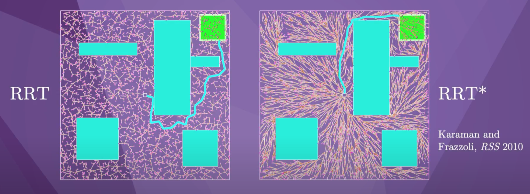
Because of their relative simplicity and explorative nature, RRTs are a popular path planning sampling algorithm. They don’t guarantee an optimal solution, however, there is an extension to the RRT algorithm called RRT* that does. This algorithm continuously updates the tree so that the solution trends toward the optimal solution as the number of nodes in the tree approaches infinity. Here’s a side-by-side of the RRT and RRT* solutions on the same problem.
Maybe in a future project I will modify my RRT implementation to include the RRT* algorithm so stay tuned for that.
If you missed my previous project implementing the A* Graph Search Algorithm, check it out here!
This RRT implementation in MATLAB was completed as part of the requirements for my graduate coursework in Dr. Eric Schearer’s course: Intelligent Controls. For more information about RRTs and other robotics topics, check out Kevin Lynch’s book, Modern Robotics: Mechanics, Planning, and Control as well as his corresponding YouTube series, found here.